> ## Documentation Index
> Fetch the complete documentation index at: https://confidence-auth-testing.mintlify.site/llms.txt
> Use this file to discover all available pages before exploring further.
# Metrics
> Metrics define how to aggregate your measurements.
A metric is an aggregation of a measurement across instances of an entity. A measurement typically
occurs when an instance of an entity, such as a user, interacts with some parts of the business.
Each such measurement event is then recorded in a fact table that has all the measurement
events of the business process of interest.
Confidence supports two types of metrics:
* **Average metrics** calculate the means of the treatment groups.
The calculation takes the average of the entity measurements after first aggregating within each entity.
For example, a user can have multiple data points.
In an average metric, these data points are first aggregated separately for each user, for example, by summing the data points.
In an experiment, the calculation averages the within-user aggregated measurements in each group.
The average metric is the most common type of metric.
* **Ratio metrics** calculate the ratios between the numerator and the denominator measurements in the treatment groups.
The calculation separately aggregates the numerator and denominator measurements across entities.
For example, let the numerator measurement be the number of successful searches, and the denominator
measurement be the number of searches.
The two measurements measure the user entity.
The ratio metric calculates the ratio of the total number of successful searches to the total number of searches.
### Choosing Between Average Metrics, Ratio Metrics, and Entity Relations
**Use Average Metrics when:**
* Analyzing at the same level as randomization (user-level metrics with user randomization)
* You want the average value per entity
* Each entity has the same weight in the analysis
**Use Ratio Metrics when:**
* Analyzing at a finer granularity than randomization (order-level metrics with user randomization)
* Calculating rates or per-unit averages (click-through rate, average order value)
* You have one-to-many relationships between randomization and measurement units
**Use Entity Relation Tables when:**
* ONLY for connecting anonymous users who later authenticate
* You need to track the same user transitioning from anonymous to authenticated state
* Never for general entity mapping or metric reuse across different experiments
For more details, see [Entity Relation Tables](./entity-relation-tables).
## Filtered Metrics
Filter rows in fact tables to create more specialized metrics. For example,
create an unfiltered metric `Number of purchases` and a filtered version `Number
of purchases on mobile`. You can create filters using any combination of logical
expressions based on fact table columns.
You can only filter metrics on
measurements and dimensions available in the same fact table that you create the metric
from.
You can create filtered attributes in your own data warehouse or in the metrics
definition in Confidence.
## Time in Metrics
All metric aggregates measurements over some time window. In Confidence, you
can configure the behavior of the time window in three ways:
**Include the user in metrics results**:
1. **At the end of a window.** Example: Second and third days' consumption. Includes all consumption during the second and third days after exposure. Includes an entity in the results **at the end of their third day of exposure**.
2. **Cumulatively during a window.** Example: Second and third days' consumption. Includes all consumption during the second and third days after exposure. Includes an entity in the results **at the beginning of their second day of exposure**.
3. **Cumulatively (no window).** Example: Average order value. Includes all orders after exposure. Includes all exposed entities.
Watch this video for an overview of the different ways to handle time in metrics in 4 minutes and 34 seconds.
For logged-in, or in other ways persistent users, it often makes sense to
consider a time window. Time-window based metrics make interpretation easier,
as you can be sure that they include the same measurements (in relation to
exposure) for all entities included in the metrics results. For experiments on
short-lived entities like short-lived cookies, using windows over for example
several days makes little sense, as one user is unlikely to come back. Even
if they do, they no longer have the same identifier. In such cases,
windows are redundant.
The figure describes how to choose the time window behavior. See more details
about the trade-offs below.
### Windows-Based Metrics
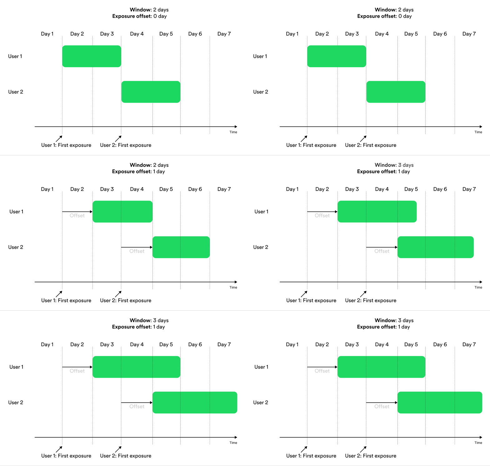
Window-based metrics measure behavior over a time window, where time is relative to exposure.
To define a window-based metric you need to specify an **exposure offset** and an **aggregation window**.
These parameters specify when the aggregation of data should start relative to exposure, and for how long the
aggregation should be applied.
Illustration of exposure offset and windows in metrics.
The benefit of window-based metrics is that they clearly define what you measure. Experiments are
often subject to novelty effects, where the effect of the treatment is strongest immediately after
exposure. By defining a time window, you have better control of when you measure the behavior you're
interested in. It treats all units in your experiment equally. If they were exposed early or late
has no bearing on the metric.
### At the End of a Window or Cumulatively During a Window
You can select two types of window-based metrics in Confidence: **At the end of a
window** and **Cumulatively during a window**.
#### At the End of a Window
Metrics that include entities in the results **At the end of a window** include
the measurements from exposed entities at the end of the window used by the metric.
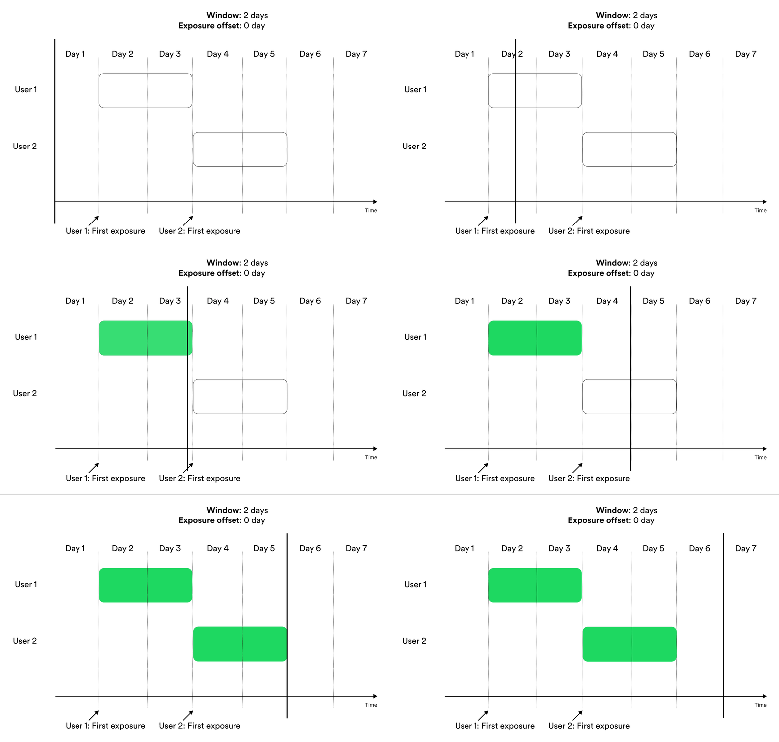
The figure illustrates how time windows work to aggregate values within
entities. The horizontal bar shows when the user was first exposed to the
experiment. The dashed part of the box is the exposure offset, and the solid
box is the aggregation window. The metric calculation includes the measurements
that fall within the aggregation window.
Illustration of including the user in metrics results at the end of a window. The metrics result at the given day of the experiment include the measurements in the green parts.
'At the end of a window' metrics show no data before `exposure offset + aggregation window - 1` time units after the start of the experiment.
For example, if you create a metric that measures user behavior during the second week after exposure, the first results
you see for the metric are available 14 days after launch. Before that day, no unit has been exposed for two weeks.
#### Cumulatively During a Window
Metrics that
include entities in the results **Cumulatively during a window** include
measurements from exposed entities cumulatively during the window.
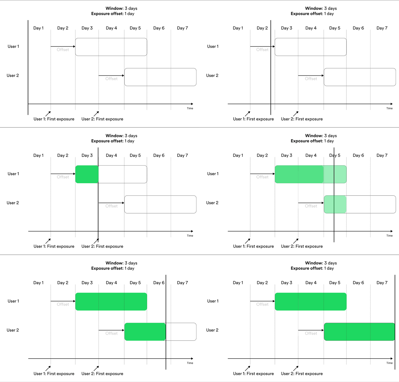
Illustration of including the user in metrics results cumulatively during a window. The metrics
result at the given day of the experiment include the measurements in the green parts.
'Cumulatively during a window' metrics show no data before
`exposure offset` time units after the start of the experiment. After that, they
show the data available for each entity in the time window. For example, if you
create a metric that measures user behavior during the second week after
exposure, the first results you see for the metric are available 7 days after
launch, at which the metric results include measurements from the eighth day of exposure
for the users exposed on the first day of the experiment.
#### Trade-Offs Between At the End of a Window and Cumulatively During a Window
Metrics that use **At the end of a window** are the most rigorous, because they include exactly the
same measurements for the entities included in the metric results at any given time. Metrics that
use **Cumulatively during a window** return results earlier because they don't need to wait for the
window to end. The downside is that they are harder to interpret as the result doesn't measure each
entity over the same length of time after exposure.
If all entities are eventually exposed for at least the upper limit of the window, the two types of
window metrics give the same results at that point. For this reason, the **Cumulatively during a
window** option offers a compromise between early results and ease of interpretation.
### Cumulatively (No Window)
Metrics that are not window-based include all measurements from all entities in the metric results
as soon as an entity is exposed. Metrics without windows are suitable when entities are short-lived,
as with for example cookie-based entities. In this case, following the same
entity over time is often difficult which makes metric windows redundant.
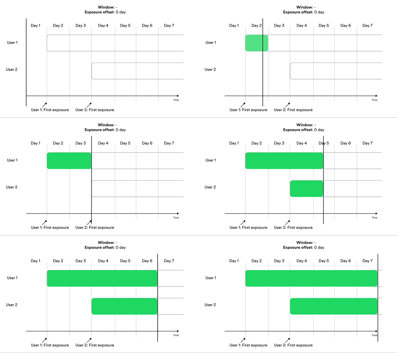
Illustration of including the user in metrics cumulatively without any window.
In cumulative metrics (without window), some entities are always measured
over longer periods than others due to that not all entities are exposed at the
same time. This makes these metrics hard to interpret. Only use these metrics
when entities are short-lived.
## Average Metrics
An average metric measures the average value across the different entities.
Typically, you have multiple facts measured within an entity.
You must select what aggregation to apply within the entity before calculating the average across entities.
Examples of average metrics include:
| Metric | Description |
| :------------------------------ | :--------------------------------------------------------------------------------------------------------------------------- |
| Average minutes played per user | Sum the minutes played for each user, then average across users |
| Share of users that were active | Count the number of events per user and map to 1 if the user was active and 0 otherwise, then average across users |
| Conversion rate | Count the number of conversion events per user and map to 1 if the user converted and 0 otherwise, then average across users |
### Within-Entity Aggregation
You can select to aggregate multiple facts within entities using one of:
| Aggregation | Description |
| :------------------------- | :----------------------------------------------------------------------- |
| Average | Average of the non-null values |
| Count | Count the non-null values |
| Count distinct | Count the number of distinct non-null values |
| Approximate count distinct | Approximate count of distinct non-null values from a HyperLogLog sketch. |
| Sum | Sum of the values |
| Max | Maximum of the non-null values |
| Min | Minimum of the non-null values |
The below examples use these facts.
| Entity | Value |
| :----- | :---- |
| A | 1 |
| A | 3 |
| A | 8 |
| A | null |
| B | 3 |
| B | 1 |
| B | 29 |
The average calculates the average of the non-null within entity values. The example table would result in
| Entity | Value |
| :----- | :---- |
| A | 4 |
| B | 11 |
The metric value is (4 + 11)/2 = 7.5.
Count counts the non-null within entity values. The example table would result in
| Entity | Value |
| :----- | :---- |
| A | 3 |
| B | 3 |
The metric value is (3 + 3)/2 = 3.
Count distinct counts the number of distinct non-null within-entity values. The example table would result in
| Entity | Value |
| :----- | :---- |
| A | 3 |
| B | 3 |
The metric value is (3 + 3)/2 = 3.
Approximate count distinct uses a HyperLogLog sketch to approximate the number of distinct non-null within-entity values. This aggregation is only available for HLL measurement columns. For example, given HLL sketch values `{seen:['id1']}` for entity A and `{seen:['id2', 'id3']}` for entity B, the result would be approximately
| Entity | Value |
| :----- | :---- |
| A | 1 |
| B | 2 |
The metric value is approximately (1 + 2)/2 = 1.5.
Max calculates the max of the non-null within entity values. The example table would result in
| Entity | Value |
| :----- | :---- |
| A | 8 |
| B | 29 |
The metric value is (8 + 29)/2 = 18.5.
Min calculates the min of the non-null within entity values. The example table would result in
| Entity | Value |
| :----- | :---- |
| A | 1 |
| B | 1 |
The metric value is (1 + 1)/2 = 1.
Sum calculates the sum of the within entity values. The example table would result in
| Entity | Value |
| :----- | :---- |
| A | 12 |
| B | 33 |
The metric value is (12 + 33)/2 = 22.5.
## Ratio Metrics
Ratio metrics aggregate the numerator and denominator separately across all entities, without first aggregating within entities. Ratio metrics differ from average metrics, which first aggregate within each entity.
### When to Use Ratio Metrics
Use ratio metrics when:
* Your unit of analysis is more granular than your randomization unit
* You want to analyze metrics at the order, session, or page view level while randomizing at the user level
* You need to calculate metrics like average order value or click-through rate
* You have one-to-many relationships between your randomization unit and measurement unit
**Example scenario**: if you randomize by users but want to calculate average pickup time per order:
* Use a ratio metric with `SUM(pickup_time) / COUNT(order_id)`
* This correctly accounts for users having different numbers of orders
* The variance calculation properly handles the user-level randomization
**Note**: Ratio metrics differ from entity relation tables, which only connect anonymous to authenticated users. If you're trying to analyze orders while randomizing on users, use ratio metrics, not entity relation tables.
Examples of ratio metrics include:
| Metric | Description |
| :------------------ | :--------------------------------------------------------------------------------------------------------------------------- |
| Click-through rate | Sum a binary measurement indicating a click in the numerator, count the number of events, or impressions, in the denominator |
| Average order value | Sum the order value in the numerator, count the number of orders in the denominator |
### Numerator and Denominator Aggregations
You can select to aggregate multiple facts for the numerator and denominator using one of:
| Aggregation | Description |
| :------------------------- | :----------------------------------------------------------------------- |
| Average | Average of the non-null values |
| Count | Count the non-null values |
| Count distinct | Count the number of distinct non-null values |
| Approximate count distinct | Approximate count of distinct non-null values from a HyperLogLog sketch. |
| Sum | Sum of the values |
| Max | Maximum of the non-null values |
| Min | Minimum of the non-null values |
The below examples use these facts.
| Entity | Measurement A | Measurement B |
| :----- | :------------ | :------------ |
| A | 1 | 8 |
| A | 3 | 3 |
| A | 8 | 2 |
| A | null | 3 |
| B | 3 | 9 |
| B | 1 | 1 |
| B | 29 | 2 |
#### Numerator
The numerator examples use measurement A from the example table above.
The average calculates the average of the non-null within entity values. The example table would result in
| Entity | Value |
| :----- | :---- |
| A | 4 |
| B | 4 |
The numerator value is 4 + 11 = 15.
Count counts the non-null within entity values. The example table would result in
| Entity | Value |
| :----- | :---- |
| A | 3 |
| B | 3 |
The numerator value is 3 + 3 = 6.
Count distinct counts the number of distinct non-null within-entity values. The example table would result in
| Entity | Value |
| :----- | :---- |
| A | 3 |
| B | 3 |
The numerator value is 3 + 3 = 6.
Approximate count distinct uses a HyperLogLog sketch to approximate the number of distinct non-null within-entity values. This aggregation is only available for HLL measurement columns. For example, given HLL sketch values `{seen:['id1']}` for entity A and `{seen:['id2', 'id3']}` for entity B, the result would be approximately
| Entity | Value |
| :----- | :---- |
| A | 1 |
| B | 2 |
The numerator value is approximately 1 + 2 = 3.
Max calculates the max of the non-null within entity values. The example table would result in
| Entity | Value |
| :----- | :---- |
| A | 8 |
| B | 29 |
The numerator value is 8 + 29 = 37.
Min calculates the min of the non-null within entity values. The example table would result in
| Entity | Value |
| :----- | :---- |
| A | 1 |
| B | 1 |
The numerator value is 1 + 1 = 2.
Sum calculates the sum of the within entity values. The example table would result in
| Entity | Value |
| :----- | :---- |
| A | 12 |
| B | 33 |
The numerator value is 12 + 33 = 45.
#### Denominator
The denominator examples use measurement B from the example table above.
The average calculates the average of the non-null within entity values. The example table would result in
| Entity | Value |
| :----- | :---- |
| A | 4 |
| B | 4 |
The denominator value is 4 + 4 = 8.
Count counts the non-null within entity values. The example table would result in
| Entity | Value |
| :----- | :---- |
| A | 4 |
| B | 3 |
The denominator value is 4 + 3 = 7.
Count distinct counts the number of distinct non-null within-entity values. The example table would result in
| Entity | Value |
| :----- | :---- |
| A | 3 |
| B | 3 |
The numerator value is 3 + 3 = 6.
Approximate count distinct uses a HyperLogLog sketch to approximate the number of distinct non-null within-entity values. This aggregation is only available for HLL measurement columns. For example, given HLL sketch values `{seen:['id1']}` for entity A and `{seen:['id2', 'id3']}` for entity B, the result would be approximately
| Entity | Value |
| :----- | :---- |
| A | 1 |
| B | 2 |
The denominator value is approximately 1 + 2 = 3.
Max calculates the max of the non-null within entity values. The example table would result in
| Entity | Value |
| :----- | :---- |
| A | 8 |
| B | 9 |
The numerator value is 8 + 9 = 17.
Min calculates the min of the non-null within entity values. The example table would result in
| Entity | Value |
| :----- | :---- |
| A | 2 |
| B | 1 |
The numerator value is 2 + 1 = 3.
Sum calculates the sum of the within entity values. The example table would result in
| Entity | Value |
| :----- | :---- |
| A | 16 |
| B | 12 |
The numerator value is 16 + 12 = 28.
#### Ratio
Assume that measurement A measures some aspect of a click and is non-null if the entity (like a visitor or a user) clicked.
Measurement B measures the corresponding impression and some aspect of it.
To calculate a click-through rate, use a count aggregation for the numerator and a count aggregation for the denominator.
The ratio is the number of clicks divided by the number of impressions, which equals (3 + 3)/(4 + 3) = 6/7.
Assume that measurement A measures the order value, with null values indicating no completed order.
To calculate the average order value, use a sum aggregation for the numerator and a count aggregation for the denominator.
Use measurement A for both. The average order value is (12 + 33)/(3 + 3) = 45/6.
## Metric Parameters
### Aggregation Window
The aggregation window controls the size of the window to include facts from. This time is always relative to
the time of exposure for the entity. Confidence only calculates metrics for an entity at the end of the window.
For example, if the aggregation window is 1 hour, an entity exposed on 14:50 would find facts between
14:50 and 15:50.
Use aggregation windows that are compatible with the frequency of your facts.
For example, you shouldn't use hourly windows if your fact table has facts
with a frequency of one per day.
### Exposure Offset
You can optionally move the window of aggregation with an offset from the time of exposure.
Sometimes the effect that you want to measure is not the effect of recently seeing the new feature, but instead
how your entities react to the new feature after some more time has passed.
### Variance Reduction With CUPED
Confidence applies [variance reduction](/docs/experiments/stats/variance-reduction) (commonly referred to as CUPED) by default.
You can turn it off, or change the aggregation window used.
The facts from before the time of exposure make it possible to reduce the variance of the metric.
By default, Confidence includes the facts that occurred one aggregation window before exposure.
Variance reduction leverages pre-exposure data to reduce the variance and increase
the signals in the metrics you select. [Deng et al. (2013)](https://dl.acm.org/doi/10.1145/2433396.2433413)
popularized this approach, commonly
referred to as CUPED, which is a form of adjustment using data collected before exposure.
The result of this adjustment is a reduction in the variance of the metric and, by extension,
the uncertainty in the estimate of the treatment effect. You can use variance reduction for
both average metrics and ratio metrics.
You should always use variance reduction, as it leads to a better and more
precise answer to the question of what the effect of the treatment was.
### Cap Values
You can cap the values of the metric to a certain range. Use this to reduce the
influence of outliers. The cap trims the metric value for each entity at the
given values. For example, a user metric that caps the maximum value at 100
replaces all user values that exceed 100 with 100. The replacement occurs after
the aggregation of the metric values for each entity, but before aggregating the
metric across entities. For example, consider a metric that sums order value for
each user. If the metric caps the maximum value at 100, the cap applies to each
user's total order value and replaces total order values that exceed 100 with
100\.
## Related Resources
Step-by-step metric creation guide
Verify your metrics work correctly
Configure measurement data sources
Improve metric precision with CUPED
 ### Windows-Based Metrics
Window-based metrics measure behavior over a time window, where time is relative to exposure.
To define a window-based metric you need to specify an **exposure offset** and an **aggregation window**.
These parameters specify when the aggregation of data should start relative to exposure, and for how long the
aggregation should be applied.
Illustration of exposure offset and windows in metrics.
### Windows-Based Metrics
Window-based metrics measure behavior over a time window, where time is relative to exposure.
To define a window-based metric you need to specify an **exposure offset** and an **aggregation window**.
These parameters specify when the aggregation of data should start relative to exposure, and for how long the
aggregation should be applied.
Illustration of exposure offset and windows in metrics.
 The benefit of window-based metrics is that they clearly define what you measure. Experiments are
often subject to novelty effects, where the effect of the treatment is strongest immediately after
exposure. By defining a time window, you have better control of when you measure the behavior you're
interested in. It treats all units in your experiment equally. If they were exposed early or late
has no bearing on the metric.
### At the End of a Window or Cumulatively During a Window
You can select two types of window-based metrics in Confidence: **At the end of a
window** and **Cumulatively during a window**.
#### At the End of a Window
Metrics that include entities in the results **At the end of a window** include
the measurements from exposed entities at the end of the window used by the metric.
The benefit of window-based metrics is that they clearly define what you measure. Experiments are
often subject to novelty effects, where the effect of the treatment is strongest immediately after
exposure. By defining a time window, you have better control of when you measure the behavior you're
interested in. It treats all units in your experiment equally. If they were exposed early or late
has no bearing on the metric.
### At the End of a Window or Cumulatively During a Window
You can select two types of window-based metrics in Confidence: **At the end of a
window** and **Cumulatively during a window**.
#### At the End of a Window
Metrics that include entities in the results **At the end of a window** include
the measurements from exposed entities at the end of the window used by the metric.
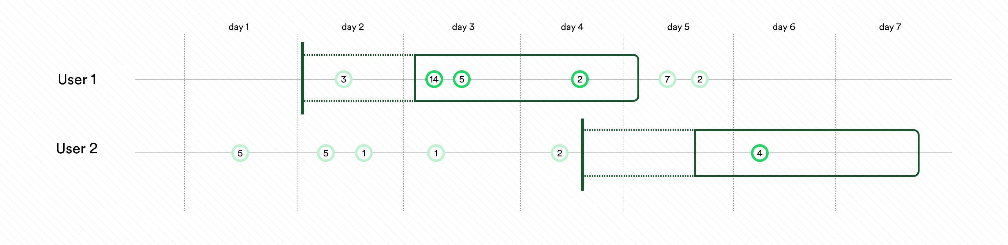 The figure illustrates how time windows work to aggregate values within
entities. The horizontal bar shows when the user was first exposed to the
experiment. The dashed part of the box is the exposure offset, and the solid
box is the aggregation window. The metric calculation includes the measurements
that fall within the aggregation window.
Illustration of including the user in metrics results at the end of a window. The metrics result at the given day of the experiment include the measurements in the green parts.
The figure illustrates how time windows work to aggregate values within
entities. The horizontal bar shows when the user was first exposed to the
experiment. The dashed part of the box is the exposure offset, and the solid
box is the aggregation window. The metric calculation includes the measurements
that fall within the aggregation window.
Illustration of including the user in metrics results at the end of a window. The metrics result at the given day of the experiment include the measurements in the green parts.